GAN
2025-07-24
1. Introduction
- The research area covered by the paper
- Training Archtecture
- Image generation
- Contributions
- The authors design an architecture of adversarial nets that G and D; a generative model Q and a discriminative model D.
- G captures the data distribution
- D estimates the probability that a sample came from the training data rather than G
- G maximizes the probability of D making a mistake
2. Methodology
Main Idea
(본문 내용) The generative model can be thought of as analogous to a team of counterfeiters, trying to produce fake currency and use it without detection, while the discriminative model is analogous to the police, trying to detect the counterfeit currency. Competition in this game drives both teams to improve their methods until the counterfeits are indistiguishable from the genuine articles.
notations:
G(z;theta_g): Generator with parameter theta_g D(x;theta_d): Discriminator with parameter theta_d
The goal is to learn the generator’s distribution over data samples.
This is a quite good figure to understand the training concept of adversarial nets.
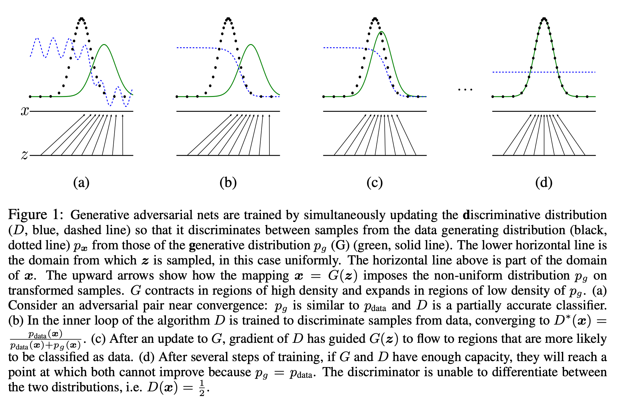
Value Function V(G,D)

D(x) is the estimate of the probability that x is a real data sample from the true data distribution.
1 - D(G(z)) is the probability that the discriminator thinks the sample is fake.
Training Algorithm
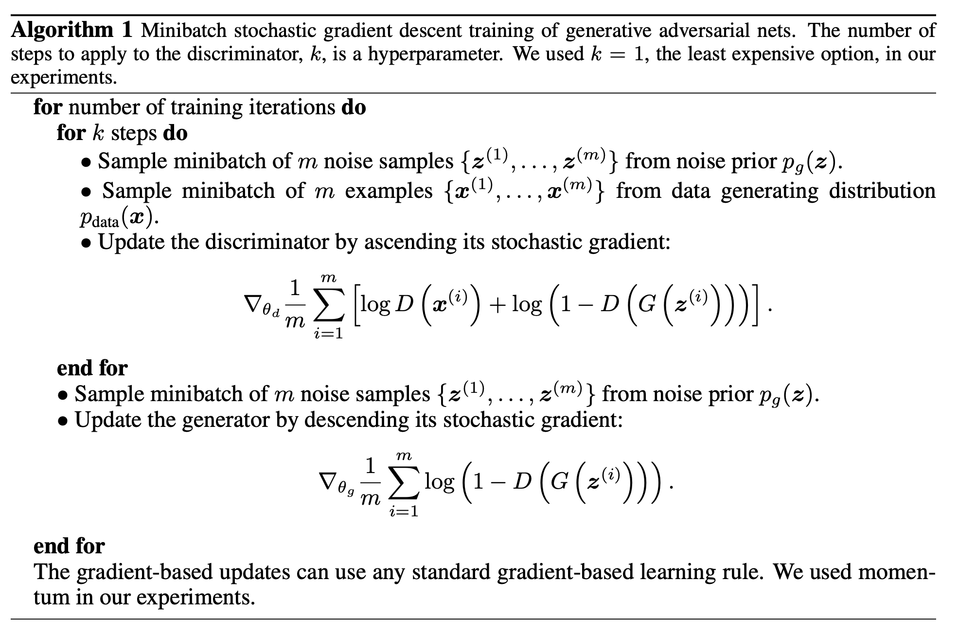
It updates the D for k steps first, then does the G, where the way is explained above the Figure 1.
- Early stage of learning, G is so poor that D can reject samples with high confidence.
- log(1 - D(G(z))) is saturates
- we can train G to maximize log(D(G(z)), rather than training G to minimize log(1-D(G(z))).
- b. gives the generator stronger gradients when it is still producing poor samples.
They show that the value function and the algorithm make G and D optimal states.
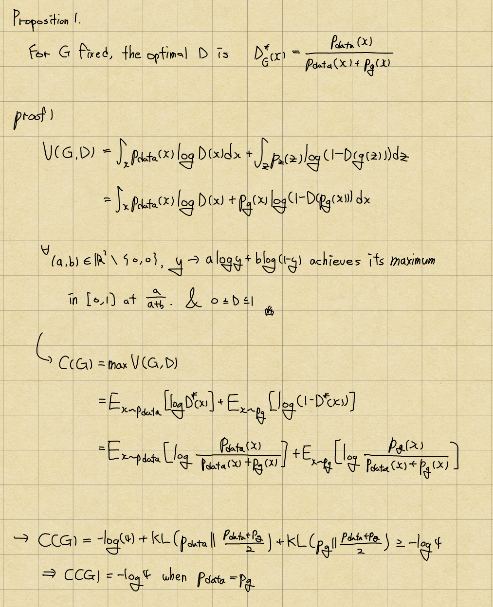
It shows that D can reach to D^*, which is optimal value. Therefore, C(G) could be minimum when p_data equals p_g.
We need to one more proposition to verify that C(G) can converge to global minimum to make p_g equal to p_data, mentioned on the above.
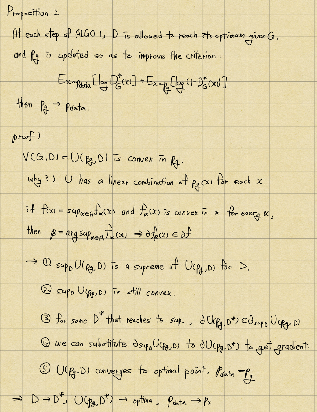
Done!
Contribution
They suggest the architecture of adversarial nets, which have been used in the ML field widely and frequently due to its simplicity.
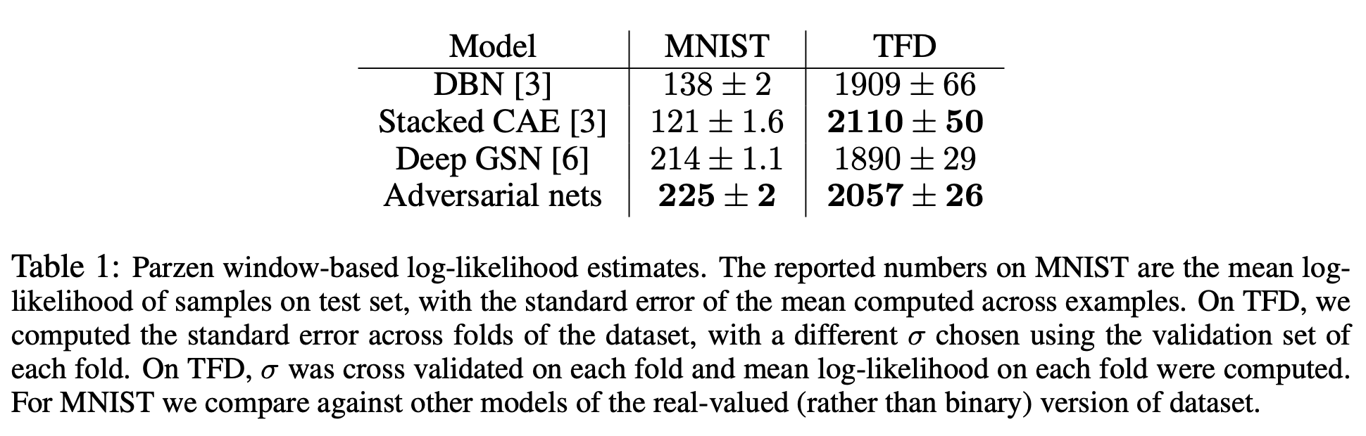
3. Experiments and Results
Dataset
MNIST(Modified National Institute of Standards and Technology): handwritten digits
TFD(Toronto Face Database): a facial expression recognition
Baseline
DBN(Deep Belief Network): composed of multiple layers of Restricted Boltzmann Machines(RBMs)
Stracked CAE(Convolutions Autoencoder): multiple convolutional autoencoders
Deep GSN(Deep Generative Stochastic Network): ?
결과
4. Conclusions
https://github.com/goranikin/DSBA-intern-study/tree/main/GAN
Scratch로 GAN 구현을 했는데, VAE때와 다르게 print로 출력되는 loss가 요동치는 것을 확인. wandb로 찍어보니…
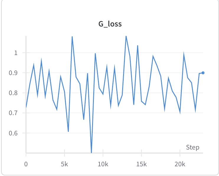
epoch 30과 50의 결과. 그닥 다를 것도 없다. 굳이 50번까지 갈 필요는 없는 것 같기도.
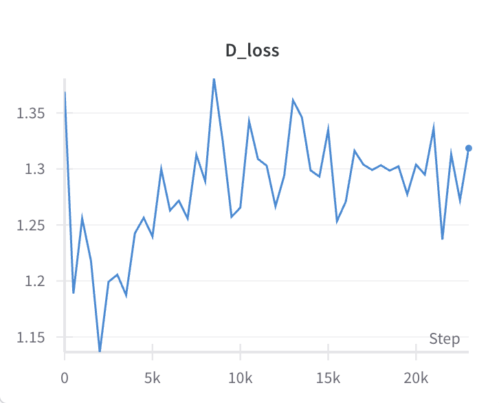
논문에서는 G에 gradient를 적용하기 전, D를 k번 학습시키는 알고리듬으로 설명했다. 다만 대부분의 구현에서는 k=1 이었는데 이것 때문인가 싶어 k=4로 늘려본 결과.
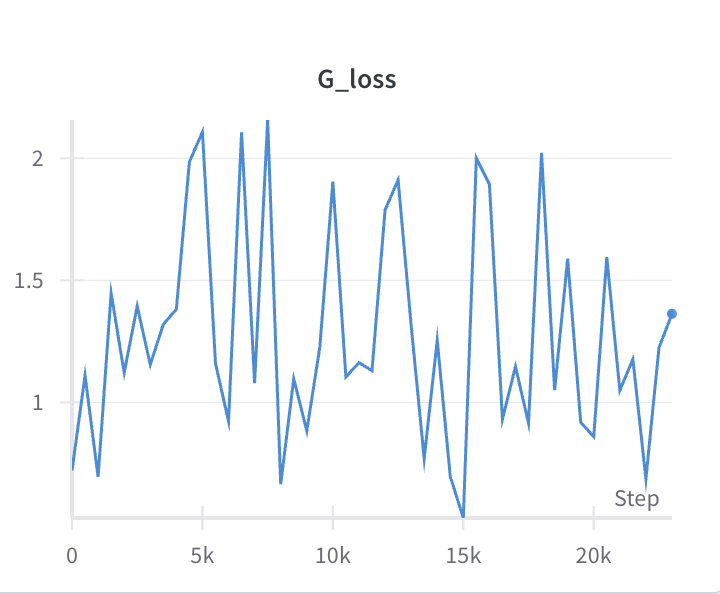
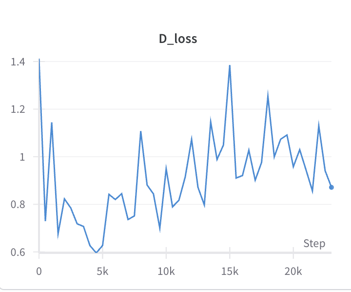 오히려 y-scale이 늘어남…
실제로 생성한 샘플들을 눈으로 보는데, 15000 steps보다 G_loss가 높은 마지막 step이 그렇게 구린 것도 아니어서… 잘 모르겠다. FID score를 찍어보려 했는데 ImageNet을 기반으로 만들어진 평가 방법이라 해상도든 뭐든 MNIST와는 거리 가 좀 먼 metric이라 판단.
- Adversarial Learning architecture를 추상적으로 Generator와 Discriminator로만 알고 있었다가 제대로 보니까 또 다름을 느낌.
- 정확히 어떤 식으로 Loss를 설정했는지
- 해당 loss의 이론적 근거
- ‘두 모델이 서로에게서 배운다’는 추상적인 사고가 매우 매력적이고, 어떤 레이어를 갖다 놓든 Generator와 Discriminator라는 개념 자체는 변하지 않으므로… 지금까지 그렇게 다양한 변형이 왜 생겼는지 알 것 같았다. 물론 기본적으로 성능이 좋은 것도 있겠지만.