VAE

Reference: Youtube
blog (in Korean)

Implementation from scratch: GitHub

---

1. Introduction

1. The research area covered by the paper

• image generation
• latent representation
• autoencoders

2. Limitations of previous studies in this task

• Limitations of existing generative models such as RBM (Restricted Boltzmann Machine), DBN (Deep Belief Network), and GMM (Gaussian Mixture Model) By GPT-4.1:
• Training these models is difficult.
• Inference becomes intractable as model size increases.
• Sampling is slow and often produces low-quality results

3. Contributions

The authors claim two main contributions:

1. A reparameterization of the variational lower bound (which makes the ELBO)
2. A posterior inference can be made especially efficient by fitting an approximate inference model

2. Related Work

RBM, GMM, DBN... and there are algorithms or mathematical backgrounds for this paper.

3. Methodology

Main Idea

Each data point is assumed to be independnet and sampled from the same distribution, and there exists a unique latent variable corresponding to each data point. The data is generated from this latent variable.

(본문 내용) We assume that the data are generated by some random process, involving an unobserved continuous random variable z.

Assumption:

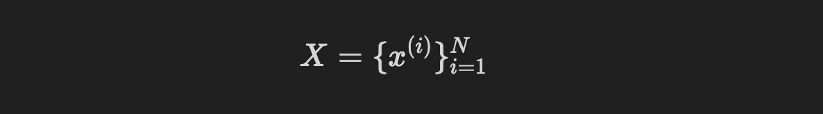
i.i.d. dataset consist of N samples:

Unobserved random variable: z

prior distribution: p_theta(z)

conditional distribution(likelihood) to generate x: p_theta^*(x|z)

→ All they are come from parametric distribution of theta.

Problem

Why?)

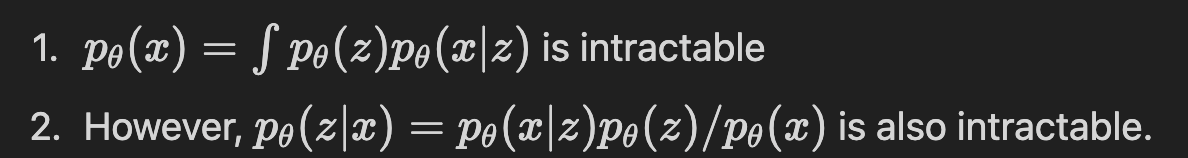
We use a neural network to generate the latent representations (z) through training. However, because the model represents a highly complex non-linear function, there is no closed-form solution for the required integration—it is analytically intractable.

Three solutions proposed by the authors are following:

1. We can’t maximize p_theta(x) directly during training theta → Maximize the ELBO
2. We can’t estimate true posterior p_theta(z|x) → an Approximate neural network q_phi(z|x)
3. We can’t estimate true p_theta(x) → Approximating with ELBO and sampling

recab

1. We want to generate image data x using a model with parameters theta.
2. We cannot directly calculate the marginal likelihood, which is the distribution from which the model generates data. (Since a neural network model is a non-linear function and does not have a closed-form solution for integration, it is impossible to obtain the loss required for backpropagation.)
3. Therefore, we do not have any information about the distribution of the latent representation z.

-> How to solve them?

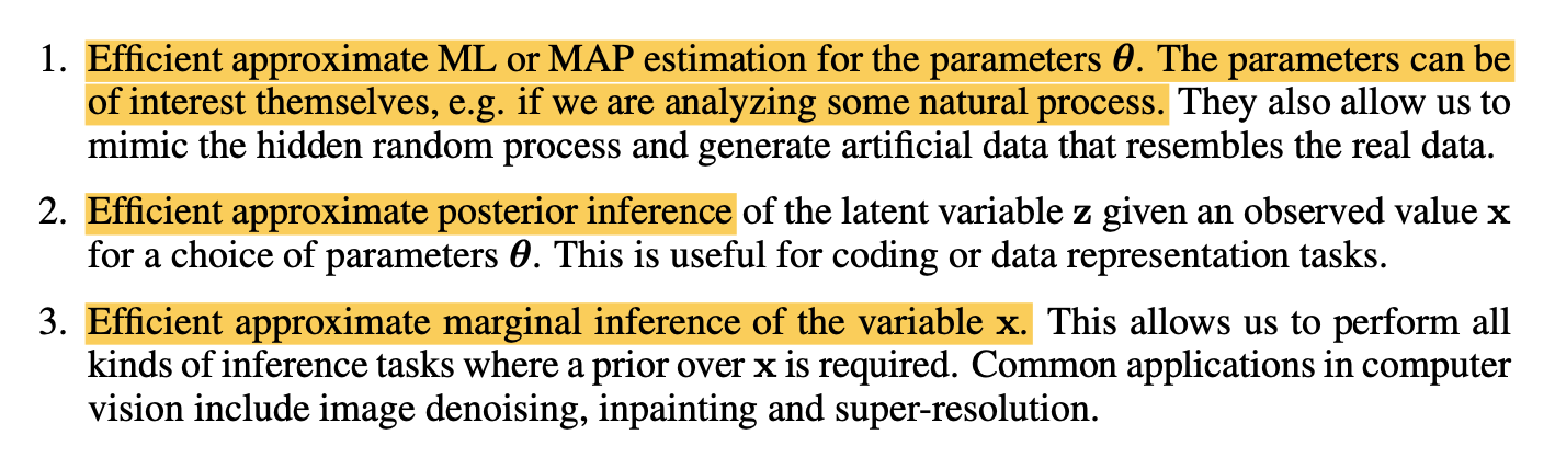
1. By maximizing the objective function ELBO, the parameters can be trained indirectly.
2. The posterior is approximated using an encoder neural network to estimate (z) from (x).
3. Ultimately, we can approximate the marginal likelihood using the ELBO.

First, we use q_phi(z|x) to approximate the porsterior, and then we train the model so that its distribution p_theta(z|x) matches this approximation.

The variational bound

There are many blogs that try to explain this topic. However, what I want to ask is: why don’t they start with the KL divergence? Our goal is to minimize the KL divergence between (q) and (p), but starting from the marginal likelihood doesn’t sufficiently explain this equation.

Re-represent RHS term

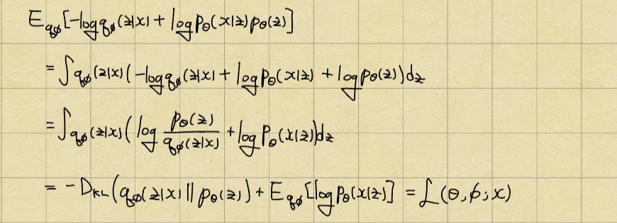
The loss what we desired! But if we look a bit more closely...

KL-D term measures how similar the distribution of (z) produced by our encoder from (x) is to the prior. The smaller this term is, the better the latent space is regularized. In VAE, we typically set the prior to a normal distribution, so this term acts as a regularizer. This is why the normal distribution is increasingly reflected in the encoder's information compression, and it helps prevent meaningless sampling when generating new images through sampling later on. This demonstrates the power of setting a prior in Bayesian methods.

The second expectation term evaluates how well the model can reconstruct (x) from the (z) produced by our encoder. Our goal is to maximize this term! (The KL-D term can be adjusted with an appropriate hyperparameter)

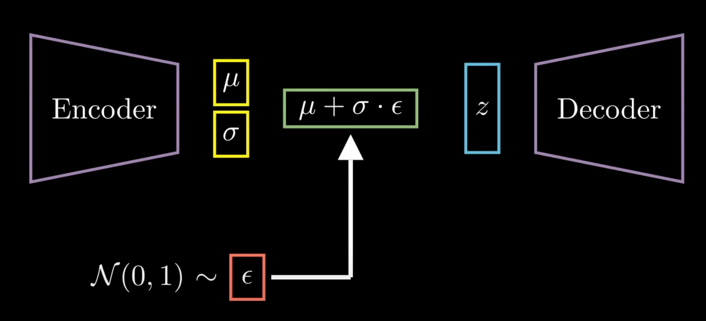
At this point, since we set the prior as a Guassian, we also set q_phi(z|x) to be Gaussian.

For each image (x), q_phi(z|x) outputs the values mu_phi and sigma_phi, which define a normal distribution. We then sample (z) from this distribution.

Q) How to backpropagate through the sampling process? (Due to randomness, the gradient is meaningless)

A) Reparameterization trick

The solution is to sampling not directly from q_phi(z|x), but instead from g_phi(epsilon, x) → then we can change integration space from z space to epsilon space

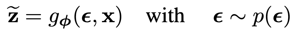
So, for a given value of epsilon, we can deterministically compute the gradient of phi w.r.t. mu and sigma! 🤘

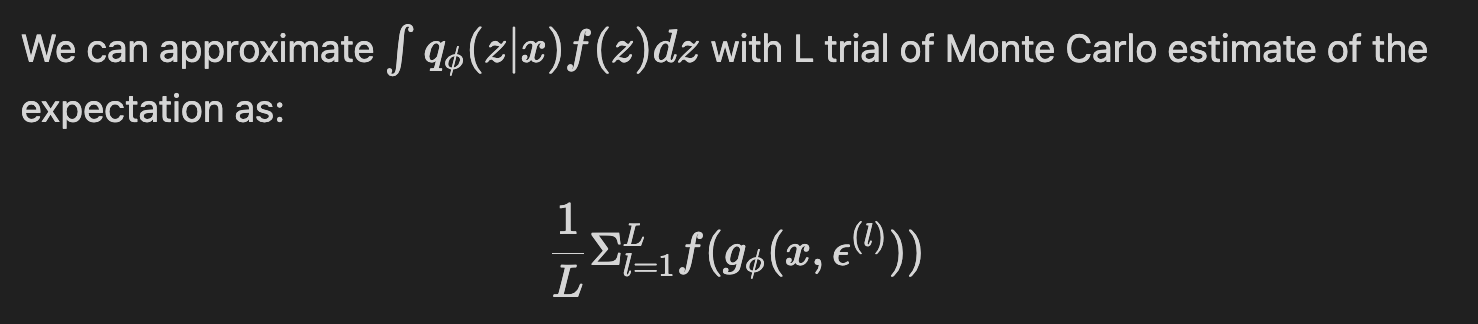
Therefore, the original expectation is approximated to Monte Carlo estimating using l samples of epsilon.

Visualization

This is pseudo code to train:

L = 5  # The number of Monte Carlo samples
recon_losses = []
for _ in range(L):
    eps = torch.randn_like(std)
    z = mu + std * eps
    x_recon = decoder(z)
    loss = F.binary_cross_entropy(x_recon, x, reduction='sum')
    recon_losses.append(loss)
recon_loss = torch.stack(recon_losses).mean()

kl_loss = -0.5 * torch.sum(1 + logvar - mu.pow(2) - logvar.exp())

total_loss = recon_loss + kl_loss
total_loss.backward()
optimizer.step()

There are a lot of ways to choose q_phi(z|x), g_phi(.), epsilon that the authors written on the paper.

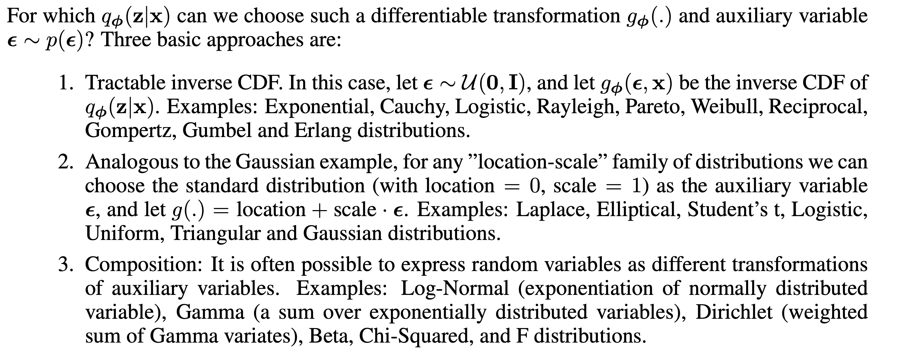
Honestly, I totally don’t have any idea of them. Also, The only method used in application is Gaussian. → I’m gonna pass!

Contribution

• A combination latent variable generation model and Autoencoder architecture
• It uses neural network which can do variational inference
• It can be applied to variety of datasets and problems

4. Experiments and Results

Datasets

• MNIST
  • handwritten digit images from 0 to 9
  • 60000 training, 10000 test
• Frey Face
  • grayscale images of a single individual’s face

Results

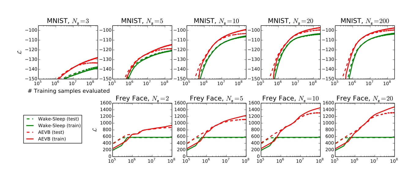
기존 Wake-Sleep algorithm보다 좋은 결과를 냈다는데… 해당 알고리듬이 뭔지 모름

1. **Wake-Sleep Algorithm이란?**

- 1995년 Geoffrey Hinton 등이 제안한 **비지도 학습(unsupervised learning)** 알고리즘이야.
- **Deep generative model**(특히 Helmholtz Machine)에서 **잠재 변수(latent variable)**를 이용해 데이터를 생성하고, 그 구조를 학습하는 데 사용됨.

---

## 2. **구조와 동작 방식**

### **모델 구성**
- **Recognition model** (또는 **inference model**):  
  데이터 \( x \)로부터 잠재 변수 \( z \)를 추정하는 모델 (VAE의 encoder와 유사)
- **Generative model**:  
  잠재 변수 \( z \)로부터 데이터를 생성하는 모델 (VAE의 decoder와 유사)

### **학습 단계**
- **Wake phase**:  
  - 실제 데이터 \( x \)를 관측
  - recognition model로 \( z \)를 추정
  - generative model의 파라미터를 업데이트 (데이터를 더 잘 생성하도록)
- **Sleep phase**:  
  - generative model에서 \( z \)를 샘플링해 \( x \)를 생성
  - recognition model의 파라미터를 업데이트 (생성된 데이터를 더 잘 인식하도록)

---

## 3. **한계점**

- **최적화가 어렵고, 근사치가 부정확할 수 있음**
- recognition model과 generative model이 따로따로 업데이트되어, 서로 잘 맞지 않을 수 있음
- 변분 하한(ELBO)을 직접적으로 최대화하지 않음

---

## 4. **VAE와의 차이점**

- **VAE는 ELBO(변분 하한)를 직접적으로 최대화**하며, 인코더/디코더를 동시에 엔드-투-엔드로 학습함
- **wake-sleep은 두 모델을 번갈아가며 따로 업데이트**함

---

## 5. **요약**

- **wake-sleep algorithm**:  
  - 고전적인 생성 모델 학습법
  - wake phase(실제 데이터 기반 학습)와 sleep phase(생성 데이터 기반 학습)로 번갈아가며 파라미터 업데이트
  - VAE보다 최적화가 덜 효율적이고, 근사치가 부정확할 수 있음

5. Conclusions

• Training latent representations with neural networks has been attempted for a long time.

  • However, VAE combines the latent variable model itself with neural networks.
  • Moreover, it allows us to observe continuous changes through interpolation in the latent space--making it interpretable!
  • Plus, after implementating the code, I found the structure to be very simple. There's nothing special: just an encoder that learns mu and sigma with a neural network, and a decoder that takes the latent representation and outputs an image.

• After reading about Diffusion models...

  • The notaiton is very different.
  • There are countless blogs explaining ELBO, but they all use exactly the same notation. It feels like everyone is copying explanations from someone who tried to make it easier to understand. The problem is, these notations are not from the VAE paper, but from Diffusion model papers. 🤔
  • I found the trick of making the probabilistic sampling distribution learnable by slightly sidestepping it very interesting. Also, making the prior a normal distribution so that the latent space generated by the parameters is mapped to the prior--this really felt like the ultimate in Bayesian thinking.

• Various ticks for estimating with Monte Carlo methods

  • But in practice, they're not really used... -> Even without multiple samples, the performance is good enough.

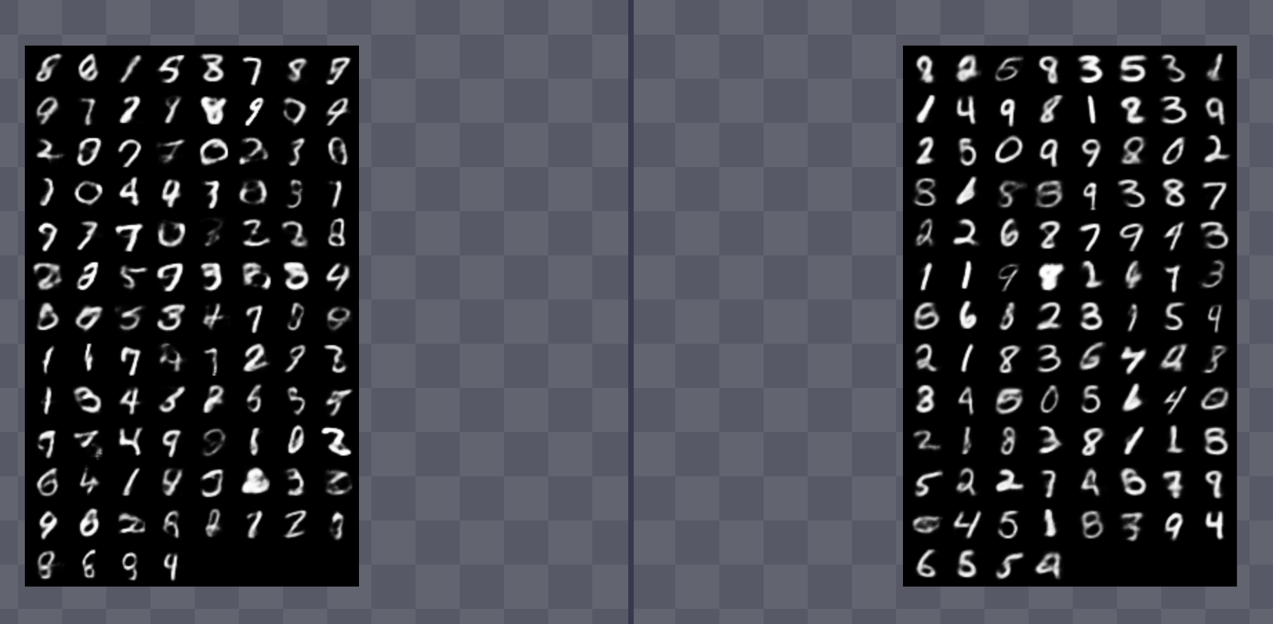
• I implemented it from scratch my self. (https://github.com/goranikin/DSBA-intern-study/tree/main/VAE)

  • 2 layers vs 5 layers... the results seem a bit clearer?
  • 
  • Interpolation like this is also possible!
  • 

---

역시 고전은 직접 읽는 게 맞다는 생각이... VAE를 읽으니 확실히 GAN도 읽어봐야 한다는 생각이 팍팍 든다. 어차피 뭐 당장에 연구를 해야만 하는 상황도 아니고, 좀 더 근본적인 논문들을 천천히 읽어도 되는 시기인 듯하니... 차라리 이미지 생성쪽에 있는 다양한 것들을 읽어보자!